VAR
Install and import#
npm install fintech-algorithmsimport { fitVAR } from "fintech-algorithms/statistical-time-series/multivariate-systems/var";Signature#
fitVAR(values, lags, includeIntercept)Vector autoregression: every series regressed on lags of all of them. The natural model when variables move together, and the base every impulse-response and variance-decomposition result is computed from.
Parameters#
| Name | Type | Notes |
|---|---|---|
values | number[][] | Multivariate series, one row per observation and one column per variable. Column order is meaningful — everything downstream refers to variables by position. |
lags | number | Lag order. Parameters grow with the square of the number of variables, so this is where a VAR runs out of data. min: 1 · integer: true |
includeIntercept | boolean | Whether to fit a constant term. optional |
Returns#
{ intercept, coefficients, sigma_u_mle, residuals, fitted, one_step_forecast, effective_observations, … }
Coefficients and the residual covariance, which is the input to structural identification.
Errors#
- When observations are fewer than the parameters to estimate — throws
Complexity: time O(n × (k × lags)²),
space O((k × lags)²).
Worked example#
executed Captured by running this function on the input its own test provides. Real output of real code — but not asserted against a published figure.
Input#
[
  [-1.4163056264, -0.7075620912],
  [-1.4144491277, -0.24959813],
  [-1.915874322, -0.31233481]
]
Showing 3 of 120 elements.
1Call#
fitVAR(values, lags, includeIntercept)Returns#
object with 16 fields: intercept, coefficients, sigma_u_mle, residuals, fitted, one_step_forecast, effective_observations, variables, …
{
  "intercept": [-0.070907764383, -0.013615076949],
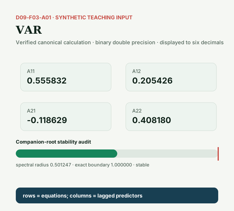
  "coefficients": [
    [
      [0.555831819774, 0.20542641337],
      [-0.118628539474, 0.408179850969]
    ]
  ],
  "sigma_u_mle": [
    [0.726815513707, 0.33092608263],
    [0.33092608263, 0.420249111781]
  ],
  "residuals": [
    [-0.410961687007, -0.115184732022],
    [-1.00749667636, -0.364632839724],
    [-0.403977225473, -0.149480679886]
  ],
  "fitted": [
    [-1.003487440693, -0.134413397978],
    [-0.90837764564, 0.052298029724],
    [-1.199973495027, 0.086173519486]
  ],
  "one_step_forecast": [0.452328292866, -0.113742494174],
  "effective_observations": 119,
  "variables": 2,
  "lags": 1,
  "row_sum_stability_bound": 0.761258233144,
  "companion_spectral_radius": 0.501247229166,
  "stability_state": "stable",
  "stability_boundary": 1,
  "near_boundary_threshold": 0.9
}
Showing 14 of 16 fields.
Other exports#
This module also exports
companionMatrix, companionSpectralRadius, choleskyLower, fitRecursiveSVAR, fitVECMFixedBeta, movingAverageMatrices, impulseResponses, forecastErrorVarianceDecomposition. Every module additionally exports run as an alias of its
primary function, and a meta object carrying its catalog id, domain, family,
shape and article URL.
Diagrams#
Calculation flow#
VAR system flow
flowchart LR
    A["Aligned stationary rows"] --> B["Lagged design matrix"]
    B --> C["Equation-wise OLS"]
    C --> D["A matrices and residual covariance"]
    D --> E["Forecast plus diagnostics"]
How it works#
This page states the contract — how to call it correctly. The article explains the concept: why it works, and where it breaks.
References#
- statsmodels vector autoregression documentation — statsmodels developers
- statsmodels VAR API documentation — statsmodels developers
- Time Series Analysis — James D. Hamilton
- New Introduction to Multiple Time Series Analysis — Helmut Lütkepohl
- Macroeconomics and Reality — Christopher A. Sims
- Statistical Analysis of Cointegration Vectors — Søren Johansen
- Publication boundary